Pie charts– represent a circle divided into sectors (cake), and are used to show the relative value that makes up a single whole. The largest sector of the circle should be the first one clockwise from the top. Each sector of the circle must be labeled (name, value and percentage are required). If it is necessary to focus on a certain sector, it is separated from the rest.

The pie chart type is useful when you want to display the share of each value in the total.

Let's build a three-dimensional pie chart that displays production load throughout the year.

Rice. Data for charting.

With the help of a pie chart, only one series of data can be shown, each element of which corresponds to a specific sector of the circle. The area of ​​the sector as a percentage of the area of ​​the entire circle is equal to the share of the row element in the sum of all elements. Thus, the sum of all shares by season is 100%. The pie chart created from this data is shown in the figure:

Rice. Pie chart.

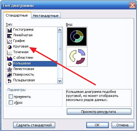
Excel provides 6 types of pie charts:

Rice. Types of pie chart.

circular – displays the contribution of each value to the total;

volumetric circular;

secondary pie – part of the values ​​of the main chart is placed on the second chart;

cut circular – sectors of values ​​are separated from each other;

volumetric cut circular;

secondary histogram – part of the values ​​of the main diagram is displayed in a histogram.

If you want to separate slices in a pie chart, you don't have to change the chart type. Simply select the circle and drag any sector away from the center. To return the chart to its original appearance, drag the sector in the opposite direction.

Rice.

It should be remembered that if you want to separate only one sector, you should make two single clicks on it. The first will select a row of data, the second – the specified sector.

Rice. Change the appearance of a pie chart.

In a pie chart, the sectors can be rotated 360 in a circle. To do this, select the tab on the ribbon Layout and point Selection Format.

A secondary pie chart, like a secondary histogram, allows some portion of the data to be displayed separately, in more detail, in a secondary chart or histogram. Moreover, the secondary diagram is taken into account in the primary diagram as a separate share. As an example, consider a chart showing sales volume for the week, where the weekend portion is plotted as a secondary pie chart. When choosing a chart type, indicate Secondary circular.

Rice. Secondary diagram.

Data that is arranged in columns and rows can be depicted as a scatter plot. A scatter plot shows relationships between numerical values ​​in multiple data series or displays two groups of numbers as a single series of x and y coordinates.

Scatter plot has two value axes, with some numerical values ​​displayed along the horizontal axis (X-axis) and others along the vertical axis (Y-axis). A scatter plot combines these values ​​into a single point and displays them at irregular intervals or clusters. Scatter plots are typically used to illustrate and compare numerical values, such as scientific, statistical, or technical data.

Good day!

Quite often, when working at a computer, you need to build some kind of graph or diagram (for example, when preparing a presentation, report, abstract, etc.),

The process itself is not complicated, but it often raises questions (even for those who have been sitting at a PC for several days). In the example below, I would like to show how to build various charts in the popular Excel program (version 2016). The choice fell on it, since it is available on almost every home PC (after all, the Microsoft Office package is still considered basic for many).

A quick way to plot a graph

What's good about the new Excel is not only that it has higher system requirements and a more modern design, but also simpler and faster graphics capabilities.

I’ll show you now how you can build a graph in Excel 2016 in just a couple of steps.

1) First, open a document in Excel on the basis of which we are going to build a graph. Typically, it consists of a plate with several data. In my case, a table with a variety of Windows operating systems.

You need to select the entire table (an example is shown in the screenshot below).

The bottom line is that Excel itself will analyze your table and offer the most optimal and visual options for its presentation. Those. you don’t have to configure anything, adjust anything, fill in data, etc. In general, I recommend it for use.

3) In the form that appears, select the type of chart that you like. I chose a classic line graph (see example below).

Actually, the diagram (graph) is ready! Now you can insert it in the form of a picture (or diagram) into a presentation or report.

By the way, it would be nice to give the diagram a name (but it’s quite simple and easy, so I won’t stop there)...

To create a pie or scatter chart (which are very visual and loved by many users), you need a certain type of data.

The point is that in order for a pie chart to clearly show the relationship, you need to use only one row from the table, and not all of them. It is clearly shown what we are talking about in the screenshot below.

Selecting a chart based on data type

So, let’s build a pie chart (screen below, see arrow numbers):

1. First, select our table;
2. then go to the section "Insert" ;
3. click on the icon ;
4. further in the list we select "Pie Chart" , click OK.

Constructing a scatter or any other chart

In this case, all actions will be similar: also select the table, in the “Insert” section, select and click on “Recommended charts”, and then select "All diagrams" (see arrow 4 in the screenshot below).

Actually, here you will see all the available charts: histogram, graph, pie, line, scatter, stock, surface, radar, tree, sunburst, box, etc. (see screenshot below). Moreover, by selecting one of the chart types, you can also choose its type, for example, select the 3-D display option. In general, choose according to your requirements...

Perhaps the only point: those charts that Excel did not recommend to you will not always accurately and clearly display the patterns of your table. Perhaps it’s worth sticking with the ones he recommends?

I have everything, good luck!

If you need to visualize difficult-to-understand data, a chart can help you with this. Using a chart, you can easily demonstrate the relationships between various indicators, as well as identify patterns and sequences in the available data.

You might think that creating a chart requires you to use difficult-to-learn programs, but that's not true. For this, a regular word text editor will be enough for you. And in this article we will demonstrate this. Here you can learn how to make a chart in Word 2003, 2007, 2010, 2013 and 2016.

How to make a chart in Word 2007, 2010, 2013 or 2016

If you are using Word 2007, 2010, 2013 or 2016, then in order to make a diagram you you need to go to the “Insert” tab and click on the “Diagram” button there.

After this, the “Insert Chart” window will appear in front of you. In this window you need to select the appearance of the diagram that you want to insert into your Word document and click on the “Ok” button. Let's take a pie chart as an example.

Once you select a chart appearance, an example of what the chart you selected might look like appears in your Word document. This will immediately open an Excel window. In Excel you will see a small table with data that is used to build a chart in Word.

To change the inserted diagram to suit your needs, you need to make changes to the table in Excel. To do this, simply enter your own column names and the necessary data. If you need to increase or decrease the number of rows in the table, you can do this by changing the area highlighted in blue.

After all the necessary data has been entered into the table, Excel can be closed. After closing Excel, you will receive the chart you need in Word.

If in the future there is a need to change the data used to construct the diagram, then for this you need to select the diagram, go to the “Design” tab and click on the “Edit data” button.

To customize the appearance of your chart, use the Design, Layout, and Format tabs. Using the tools on these tabs, you can change the chart color, labels, text wrapping, and many other options.

How to Make a Pie Chart in Word 2003

If you use the text editor Word 2003, then in order to make a diagram you you need to open the “Insert” menu and select “Drawing - Diagram” there.

As a result, a chart and table will appear in your Word document.

To make a pie chart right-click on the chart and select the “Chart Type” menu item.

After this, a window will appear in which you can select the appropriate chart type. Among other things, you can select a pie chart here.

After saving the settings for the appearance of the chart, you can start changing the data in the table. Double-click on the diagram with the left mouse button and a table will appear in front of you.

Using this table, you can change the data that is used to build the chart.

§ 1 What is a diagram?

In this lesson, you will not only learn what a pie chart is, but also learn the basic skills of creating, reading, and working with pie charts. Let's start with what is a diagram, what and where is it used?

Often in our lives, the results of human activity, for example, comparing the cost of products, the composition of various mixtures, or some other numerical data, are more convenient to present visually, in the form of a picture. It is easier to compare numerical values ​​if they are represented as graphic objects of different sizes. Drawings are better perceived by humans. Using them, you can clearly compare the results and draw certain conclusions. Such drawings are called graphs and diagrams.

Today we will get acquainted with diagrams. A diagram (from Greek “image, drawing, drawing”) is a graphical representation of data that allows you to quickly assess the relationship of several quantities.

§ 2 Types of diagrams

There are many types of diagrams known. They can be planar and volumetric. Among the diagrams there are:

etc. We will study pie charts.

§ 3 Pie chart

Pie charts are a fairly common type of chart; an integer value is depicted in such charts as a circle. And part of the whole is in the form of a sector of a circle, i.e. its part, the area of ​​which corresponds to the contribution of this part to the whole. This type of diagram is convenient to use when you need to show the share of each value in the total volume.

§ 4 How to build a pie chart?

Let's look at a specific example. An alloy of iron and tin contains 70% pure iron, the rest is tin. To visually depict this situation, let's draw a circle and paint 70% of its area red and the remaining 30% blue.

Because in a circle 180 +180=360º, then you need to find 30% of 360º. For this, 360:100 ∙ 30= 108º. This means you need to draw two radii at an angle of 108º and paint the part of the circle between them blue, and the rest of the circle red. So we have a pie chart.

More often than not, to construct a pie chart, you have to break the circle into more parts. For example, let's create a nutrition pie chart for students. For schoolchildren, the most important five meals a day is: first breakfast - 20%, second breakfast - 15%, lunch - 40%, afternoon snack - 10%, dinner - 15% of the daily diet.

First, let's find how many degrees there are in each area. Let's perform the following calculations:

1) 360: 100 ∙ 20 = 72º - this occurs at morning breakfast

2) 360: 100 ∙ 15 = 54º - second breakfast

3) 360: 100 ∙ 40 = 144º - occurs at lunch

4) 360: 100 ∙ 10 = 36º - afternoon snack

5) 360: 100 ∙ 15 = 54º - dinner

Now, in the circle we draw radii OA, OB, OS, OD and OE so that angle AOB is 72º, angle BOC is 54º, angle COD is 144º, angle DOE is 36º and angle EOA is 54º. Next, all that remains is to choose colors and paint over each area. We received a pie chart, from which it is very clearly seen that the most nutrition comes from lunch, and the least from the afternoon snack.

By the way, it should be noted that a pie chart remains visual only if the number of parts of the whole chart is small. If there are too many parts of the diagram, its use is ineffective due to the insignificant differences in the data being compared.

Thus, in this lesson you learned what a pie chart is and learned how to build them yourself.

List of used literature:

1. Mathematics 5th grade. Vilenkin N.Ya., Zhokhov V.I. and others. 31st ed., erased. - M: 2013.
2. Didactic materials for mathematics grade 5. Author - Popov M.A. - year 2013
3. We calculate without errors. Work with self-test in mathematics grades 5-6. Author - Minaeva S.S. - year 2014
4. Didactic materials for mathematics grade 5. Authors: Dorofeev G.V., Kuznetsova L.V. - 2010
5. Tests and independent work in mathematics grade 5. Authors - Popov M.A. - year 2012
6. Mathematics. 5th grade: educational. for general education students. institutions / I. I. Zubareva, A. G. Mordkovich. - 9th ed., erased. - M.: Mnemosyne, 2009. - 270 pp.: ill.

In this pie chart tutorial, you'll learn how to create a pie chart in Excel, how to add or remove a legend, how to label a pie chart, show percentages, how to split or rotate it, and much more.

Pie charts, also known as sectoral, are used to show what portion of a whole individual amounts or shares, expressed as a percentage, make up. In such graphs, the entire circle is 100%, while individual sectors are parts of the whole.

The public loves pie charts, while data visualization experts hate them, and the main reason for this is that the human eye is not able to accurately compare angles (sectors).

If you can’t completely abandon pie charts, then why not learn how to build them correctly? Drawing a pie chart by hand is difficult, with confusing percentages being a particular challenge. However, in Microsoft Excel you can create a pie chart in just a couple of minutes. Then just spend a few more minutes using the chart's special settings to give it a more professional look.

How to build a pie chart in Excel

Creating a pie chart in Excel is very easy and requires just a few clicks. The main thing is to correctly format the source data and choose the most suitable type of pie chart.

1. Prepare the initial data for the pie chart

Unlike other Excel graphs, pie charts require you to organize your raw data into a single column or row. After all, only one series of data can be constructed in the form of a pie chart.

In addition, you can use a column or row with category names. Category names will appear in the pie chart legend and/or data labels. In general, a pie chart in Excel looks best if:

• The chart contains only one data series.
• All values ​​are greater than zero.
• There are no empty rows or columns.
• The number of categories does not exceed 7-9, since too many sectors of the diagram will blur it and it will be very difficult to perceive the diagram.

As an example for this tutorial, let's try to build a pie chart in Excel based on the following data:

2. Insert a pie chart into the current worksheet

Select the prepared data and open the tab Insert(Insert) and select the appropriate chart type (we’ll talk about the different ones a little later). In this example, we will create the most common 2-D pie chart:

Advice: When highlighting your source data, be sure to select column or row headings so that they automatically appear in your pie chart titles.

3. Select a pie chart style (if necessary)

When the new pie chart appears on the worksheet, you can open the tab Constructor(Design) and in the section Chart styles(Charts Styles) Try different styles of pie charts, choosing the one that best suits your data.

The default pie chart (Style 1) in Excel 2013 looks like this on a worksheet:

Agree, this pie chart looks a little simple and, of course, requires some improvements, for example, the name of the chart, and perhaps it is worth adding more. We'll talk about all this a little later, but now let's get acquainted with the types of pie charts available in Excel.

How to Create Different Types of Pie Charts in Excel

When creating a pie chart in Excel, you can choose one of the following subtypes:

This is the standard and most popular subtype of pie chart in Excel. To create it, click on the icon Circular(2-D Pie) tab Insert(Insert) in section Diagrams(Charts).

3D pie chart in Excel

Volumetric circular(3-D Pie) charts are very similar to 2-D charts, but display data on 3-D axes.

When building a 3D pie chart in Excel, additional functions appear, such as .

Secondary Pie or Secondary Bar Chart

If a pie chart in Excel consists of a large number of small sectors, then you can create Secondary circular(Pie of Pie) chart and show these minor sectors on another pie chart, which will represent one of the sectors of the main pie chart.

Secondary ruled(Bar of Pie) is very similar to Secondary circular(Pie of Pie) chart, except that the sectors are displayed in a secondary histogram.

While creating Secondary circular(Pie of Pie) or Secondary ruled(Bar of Pie) charts in Excel, the last three categories will be moved to the second chart by default, even if those categories are larger than the others. Since the default settings are not always the most appropriate, you can do one of two things:

• Sort the raw data on the worksheet in descending order so that the smallest values ​​end up in the secondary chart.
• Choose yourself which categories should appear on the secondary diagram.

Selecting data categories for a secondary chart

To manually select data categories for a secondary chart, do this:

1. Right-click on any sector of the pie chart and select from the context menu Data series format(Format Data Series).
2. Series parameters(Series Options) in the dropdown list Split row(Split Series By) select one of the following options:
   • Position(Position) – allows you to select the number of categories that will appear in the secondary chart.
   • Meaning(Value) – allows you to define the threshold (minimum value). All categories that do not exceed the threshold will be transferred to the secondary chart.
   • Percent(Percentage value) – the same as Meaning(Value), but here the percentage threshold is indicated.
   • Other(Custom) - Allows you to select any slice from the pie chart on the worksheet and specify whether it should be moved to a secondary chart or left in the primary chart.

In most cases, a threshold expressed as a percentage is the most reasonable choice, although it all depends on the input data and personal preference. This screenshot shows the division of a series of data using a percentage indicator:

Additionally, you can configure the following parameters:

• Change Side clearance(Gap between two charts). The gap width is set as a percentage of the secondary diagram width. To change this width, drag the slider, or manually enter the desired percentage.
• Resize the secondary chart. This indicator can be changed using the parameter Second construction area size(Second Plot Size), which represents the size of the secondary plot as a percentage of the size of the main plot. Drag the slider to make the chart larger or smaller, or enter the percentages you want manually.

Donut charts

Ring A donut chart is used instead of a pie chart when more than one series of data is involved. However, in a donut chart it is quite difficult to assess the proportions between elements of different series, so it is recommended to use other types of charts (for example, a histogram).

Changing the hole size in a donut chart

When creating a donut chart in Excel, the first thing you need to do is change the size of the hole. This is easy to do in the following ways:

Customize and Improve Pie Charts in Excel

If you only need a pie chart in Excel to get a quick look at the big picture of your data, then the default standard chart is fine. But if you need a beautiful diagram for a presentation or for some similar purposes, then it can be improved somewhat by adding a couple of touches.

How to Add Data Labels to a Pie Chart in Excel

A pie chart in Excel is much easier to understand if it has data labels. Without labels, it is difficult to determine what share each sector holds. You can add labels to a pie chart for the entire series or just for a specific element.

Add data labels to pie charts in Excel

Using this pie chart as an example, we'll show you how to add data labels for individual slices. To do this, click on the icon Chart elements(Chart Elements) in the upper right corner of the pie chart and select the option Data Signatures(Data Labels). Here you can change the location of the signatures by clicking on the arrow to the right of the parameter. Compared to other chart types, pie charts in Excel provide the most choice in label placement:

If you want the labels to appear inside callouts outside the circle, select Data callout(Data Callout):

Advice: If you decide to place labels inside the chart sectors, please note that the default black text is difficult to read against the background of a dark sector, as, for example, is the case with the dark blue sector in the picture above. To make it easier to read, you can change the signature color to white. To do this, click on the signature, then on the tab Format(Format) press Fill text(Text Fill). In addition, you can change .

Categories in data labels

If a pie chart in Excel consists of more than three slices, then labels can be added directly to each slice so as not to force users to jump between the legend and the chart to find information about each slice.

The fastest way to do this is to select one of the ready-made layouts in the tab Constructor > Chart Layouts > Express Layouts(Design > Chart Styles > Quick Layout). Layout 1 And Layout 4 contain category names in data labels:

To access other options, click the icon Chart elements(Chart Elements) in the upper right corner of the pie chart, click on the arrow next to the item Data Signatures(Data Labels) and select Extra options(More options). A panel will appear Data Signature Format(Format Data Labels) on the right side of the worksheet. Go to section Caption options(Label Options) and check the option Category name(Category Name).

In addition, you can take advantage of the following options:

• Under the heading Include in signature(Label Contains) select the data that should be contained in the labels. In our example this is Category name(Category Name) and Meaning(Value).
• In the dropdown list Delimiter(Separator) select how to separate the data in the captions. In our example, the separator is selected New line(New Line).
• Under the heading Mark position(Label Position) select where to place the label. In our example we selected At the edge outside(Outside End).

Advice: Now the data labels have been added to the pie chart, the legend is no longer needed and can be removed by clicking on the icon Chart elements(Chart Elements) and uncheck the box next to the item Legend(Legend).

How to Show Percentages on a Pie Chart in Excel

When the original data in a pie chart is expressed as a percentage, the signs % will appear on the diagram automatically as soon as the parameter is enabled Data Signatures(Data Labels) in the menu Chart elements(Chart elements) or parameter Meaning(Value) on the panel Data Signature Format(Format Data Labels), as shown in the example above.

If the original data is expressed in numbers, then you can show in the captions either the original values, or percentages, or both.

• Right-click on any sector of the pie chart and select from the context menu Data Signature Format(Format Data Labels).
• In the panel that appears, tick the parameters Meaning(Value) and/or Shares(Percentage) as shown in the example. Excel will calculate the percentages automatically based on the assumption that the entire pie chart is 100%.

Dividing a pie chart or highlighting individual sectors

To highlight individual values ​​in a pie chart, you can break it up, i.e. separate all sectors from the center of the diagram. You can also highlight specific sectors by moving only them away from the main diagram.

Fragmented pie charts in Excel can be in 2-D or 3-D format, and donut charts can also be split.

How to split a pie chart in Excel

The fastest way to split a pie chart in Excel is to click on the pie chart to select all the slices and then use your mouse to drag them away from the center of the chart.

To more accurately customize the pie chart layout, follow these steps:

How to highlight individual sectors of a pie chart

To draw the user's attention to a specific sector of a pie chart, you can move this sector out of the general circle of the chart.

I repeat: The fastest way to move individual sectors of the chart is to select them and move them away from the center using the mouse. To select a separate sector, you need to double-click on it.

There is another way: select the sector that you want to extend, right-click on it and click in the context menu Data series format(Format Data Series). Then in the panel that appears, open the section Series parameters(Series Options) and configure the parameter Cutting a point(Point Explosion):

Comment: If you need to select several sectors, you will need to repeat this process with each of them, as shown above. It is impossible to select several sectors of a pie chart at once in Excel, but you can split the chart completely, or select only one sector at a time.

How to Expand a Pie Chart in Excel

When creating a pie chart in Excel, the order in which the categories are drawn depends on the order of the data on the worksheet. You can rotate the pie chart 360 degrees to show data from different perspectives. Typically, a pie chart looks best if its smallest sectors are in the front.

To rotate a pie chart in Excel, you need to follow these steps:

1. Right-click on the diagram and select Data series format(Format Data Series).
2. In the panel that appears in the section Series parameters(Series Options) move the option slider Angle of rotation of the first sector(Angle of first slice) to expand the diagram, or enter the required value manually.

Rotating 3D pie charts

An option is available for 3D pie charts Rotate a volumetric figure(3-D Rotation). To access this option, you need to right-click on any sector of the diagram and select from the context menu Rotate a volumetric figure(3-D Rotation).

A panel will appear Chart Area Format(Format Chart Area), where you can configure the following parameters for rotating a volumetric figure:

• Horizontal Rotation around the X axis(X Rotation)
• Vertical Rotation around Y axis(Y Rotation)
• Viewing angle – parameter Perspective(Perspective)

Comment: Pie charts in Excel can rotate around the horizontal axis and vertical axis, but not around the depth axis (Z-axis). Therefore the parameter Rotation around the Z axis(Z Rotation) is not available.

If you click on the up or down arrows in the fields for entering rotation angles, the diagram will immediately rotate. In this way, you can make small changes in the angle of rotation of the diagram until it is in the desired position.

How to Organize Pie Chart Sectors by Size

Typically, pie charts are easier to understand if their slices are sorted from largest to smallest. The fastest way to achieve this result is to sort the source data on a worksheet. If you can’t sort the source data, you can change the arrangement of sectors in the Excel pie chart as follows:

How to change colors in a pie chart

If the standard colors of a pie chart in Excel do not suit you, there are several options:

Changing the color scheme of a pie chart in Excel

To select a different color scheme for a pie chart in Excel, you need to click on the icon Chart styles(Chart Styles), open tab Color(Color) and select the appropriate color scheme. The icon appears when a chart is selected to the right of it.

You can also click on any point in the pie chart to display a group of tabs on the Menu Ribbon Working with charts(Chart Tools) and on the tab Constructor(Design) in the section Chart styles(Chart Styles) click on the button Change colors(Change Colors):

Select colors for each sector separately

As you can see in the picture above, the choice of color schemes for charts in Excel is not rich, and if you need to create a stylish and bright pie chart, you can choose a different color for each sector. For example, if diagrams are located inside sectors, then you need to take into account that black text is difficult to read against a background of dark colors.

To change the color of an individual sector, select it by double-clicking on it with the mouse. Then open the tab Format(Format), press Filling a shape(Shape Fill) and select the desired color.

Advice: If your Excel pie chart contains a large number of small, not particularly important sectors, you can color them gray.

How to customize the appearance of a pie chart in Excel

If you are creating a pie chart in Excel for a presentation or for exporting to other applications, you can make it look more attractive.

To open formatting options, right-click on any sector of the pie chart and click in the context menu Data series format(Format Data Series). A panel will appear on the right side of the worksheet. On the tab Effects(Effects) experiment with the options Shadow(Shadow) Backlight(Glow) and Smoothing(Soft Edges).

On the tab Format(Format) Other useful formatting tools are available:

• Changes the dimensions of the pie chart (height and width);
• Changing the fill and outline of a shape;
• Using various effects for the figure;
• Using WordArt styles for text elements;
• And much more.

To use these formatting tools, select the pie chart element you want to format (legend, data label, slice, or chart title) and select the tab Format(Format). Appropriate formatting options will be active, while unneeded formatting options will be disabled.

Now that you know how to create a pie chart in Excel, let's try to compile a list of the most important recommendations that will help make it both attractive and meaningful:

• Sort sectors by size. To make the pie chart more understandable, you need to sort the sectors from large to small or vice versa.
• Group sectors. If your pie chart has a large number of slices, it is best to group them and then use separate colors and shades for each group.
• Color minor small sectors gray. If the pie chart contains small sectors (less than 2%), color them gray or group them into a separate category called Other.
• Rotate the pie chart so that the smallest sectors are in front.
• Avoid too many data categories. Too many sectors on a chart look like a clutter. If there are too many categories of data (more than 7), then separate the small categories into a secondary pie or secondary bar chart.
• Don't use a legend. Add labels directly to the slices of your pie chart so that readers don't have to jump back and forth between the slices and the legend.
• Don't get carried away with 3-D effects. Avoid a lot of 3-D effects in the diagram, as they can significantly distort the perception of information.